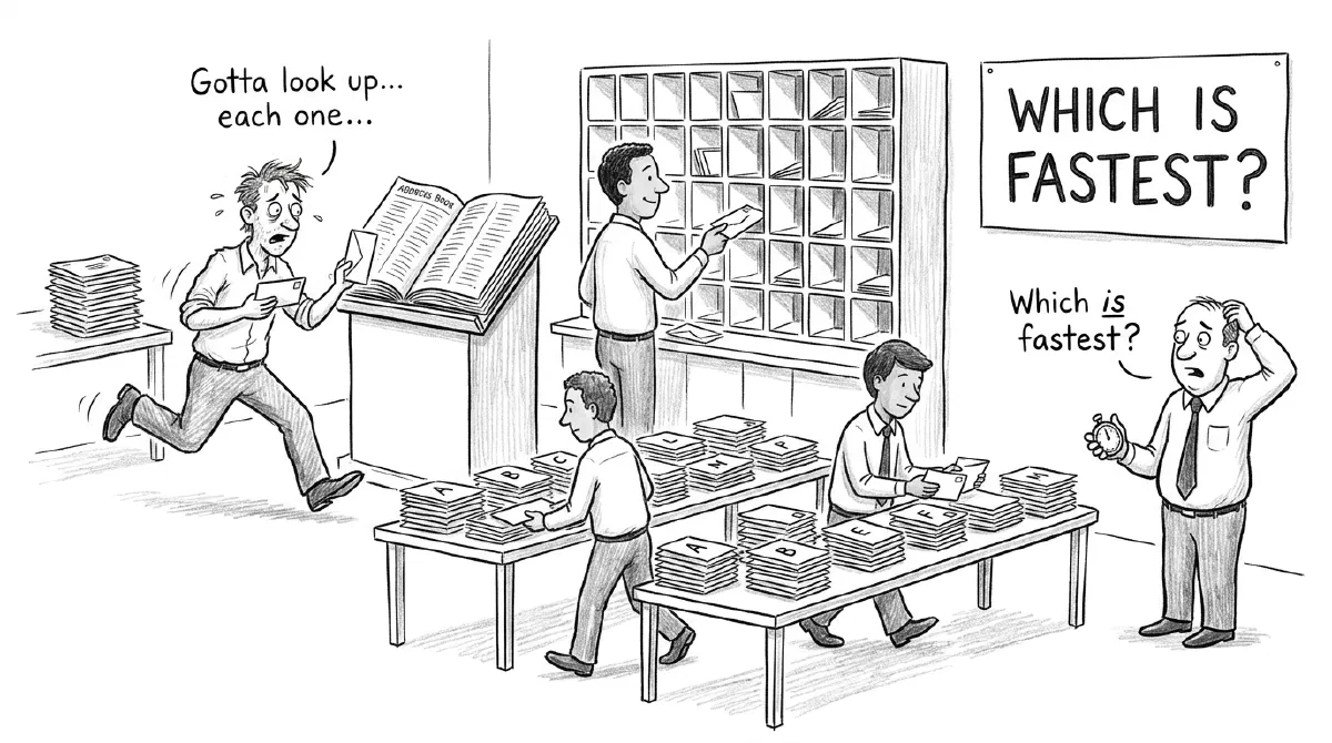
| Nested loop | Hash join | Merge join | |
|---|---|---|---|
| How it works | For each row of the first input, look up matching rows in the second | Load one input into a hash table in memory, then check every row of the other against it | Walk two inputs sorted on the join column side by side |
| What it needs | An index on the second table’s join column | Memory for the hash table (work_mem in PostgreSQL, join_buffer_size in MySQL) | Both inputs in join-column order, from an index or a sort |
| Fastest here | Under about 5,000 customers: 68 ms against 381 ms for hash at 1,000, with merge join tied because it walks the same index | Past about 5,000: 360 ms against 1,219 ms for nested loop at 20,000 | Two big tables in key order: 1,084 ms against 1,621 ms hash and 3,029 ms nested loop |
| How it fails | Cost grows with every outer row: 13.5 s at 200,000 customers, against 0.86 s for hash | Starts by reading the whole second table, so it took 268 ms even for 10 customers | Without an index to supply the order, a sort comes first |
| PostgreSQL 18 | Chosen by cost | Chosen by cost | Chosen by cost |
| MySQL 8.4 | Chosen whenever an index fits the join | Used only when no index fits the join | Does not exist |
All of it is measured below except the sort in merge join’s failure row, which is documented behavior these tests never triggered.
So here is how a join works, in outline. Looking up each row of one table in the other is the natural first answer, and with an index on the second table’s join column (a sorted copy of that column with pointers back to the rows) it is a good one, because each lookup goes straight to the few rows that match. But every lookup is a separate trip, into the index and then out to wherever those rows sit in the table, and a join that needs a large share of the table makes one such trip per row. Past some point it is cheaper to read the whole table once, front to back, and match rows as they go by. Databases do that in two ways: hold one side in a lookup table in memory and stream the other side past it, or read both sides in the same sorted order and pair them off. Counting the lookup, that makes three algorithms, called nested loop, hash join and merge join, and before each query PostgreSQL’s planner, the part that picks how a query runs, estimates the rows each step will produce, prices the options and runs the cheapest.
A quick reminder about query plans
The planner’s choice is printed in the query plan, the tree of steps the database runs to answer a query. EXPLAIN shows the plan, and EXPLAIN ANALYZE runs the query and adds what actually happened. Each step is a node, indented under the node that uses its output, and each carries two estimates: rows, how many rows the planner expects it to produce, and cost, a number in arbitrary units that only means something next to the cost of another plan. A join is a node with two children, the two inputs it matches. The habit this post leans on is reading the estimated rows against the actual ones, because the planner chose its join from the estimate; the how-tos for PostgreSQL and MySQL cover the rest of the output (MySQL calls its planner the optimizer).
Three ways to join two tables
Each of the three needs something different from its inputs, and what it needs decides how its cost grows as the inputs grow. That growth is what the planner is really comparing when it prices them.
The tests ran on PostgreSQL 18.6 and MySQL 8.4.13 in Docker with default settings, each container limited to 4 CPUs and 4 GB of memory, on the same tables as the two EXPLAIN posts: 200,000 customers and 5,000,000 orders, each order belonging to a random customer, with an index on orders.customer_id. A third table, shipments, holds one row for each of the 4,950,073 shipped orders, keyed by order id and written in order id order. PostgreSQL can split one join across several processes, and it can compile parts of a query at run time (JIT); I turned both off, as in the EXPLAIN post, so parallel joins are simplified away here. Every join is also an inner join on one equality, such as o.customer_id = c.id; outer joins and other conditions change which of the three are allowed, which this post leaves aside. Timings are medians of five runs (three for the biggest joins) with the tables already read once. Run-to-run noise between sessions was up to about 20 percent, so smaller differences mean nothing.
The query for most of this post totals the orders of the first N customers:
| |
Nested loop
A nested loop is the lookup from the outline, and what it needs is an index on the second input’s join column, because it searches that input once for every row of the first. Without one, each search would have to read the whole orders table. With 1,000 customers PostgreSQL picks it (plan trimmed to the join and its two inputs):
| |
The first child is called the outer side, and here it produces 1,000 customers. The second child, the inner side, runs once per customer (loops=1000), and each run uses the index to find that customer’s 25 or so orders. So the work grows with the outer side: twice the customers, twice the index lookups. Buffers counts pages, the 8 KB blocks PostgreSQL stores a table in, and this join touched 27,901 of them, because each customer’s orders are scattered across the table and almost every order lives on a different page.
Hash join
A hash join needs no index at all. What it needs is memory, for a hash table: a lookup structure, keyed on the join column, that it builds from one input before reading the other. Raise the limit to 20,000 customers and the plan changes to one:
| |
Read it from the bottom. The Hash node collects the 20,000 customer ids into the hash table, which took 960 kB and a millisecond. Then Seq Scan on orders reads all 5,000,000 orders once, and for each one the join checks the hash table for its customer_id. Nothing runs more than once (loops=1 everywhere), and the index on orders.customer_id is not used at all. Most of the cost is that one scan of the orders table, and it is the same whether the hash table holds 20 customers or 20,000: with only 10 customers a forced hash join still took 268 ms. The memory limit comes from work_mem in PostgreSQL and join_buffer_size in MySQL, and Batches: 1 means the hash table fit inside it. That line comes back below.
Merge join
A merge join needs both inputs sorted on the join column, either read from an index in that order or sorted first, and in return it reads each input once. The customers-and-orders query cannot get its orders in that order cheaply, as the next section shows. The shipments join can, because both it and orders have primary keys on the order id:
| |
| |
Both inputs come out of their primary key indexes already in order id order. The join reads one row from each side. If the ids match, that is a result row; if not, it moves the side with the smaller id forward. Each table is read once, front to back, with no hash table and no sort, and the Merge Cond line gives it away.
This is the case merge join exists for: two big tables, every row needed, both already in key order. Forcing the other two algorithms onto the same join shows why the planner picked it:
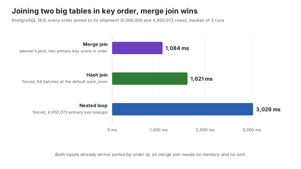
The hash join has to load 4,950,073 shipments into its hash table before it can match anything, and at the default work_mem that table did not fit, so PostgreSQL split it into 64 batches written to temporary files (Batches: 64 under the Hash node). The nested loop is less awful than its 4,950,073 lookups suggest, because it scans shipments in order id order, so consecutive lookups into the orders primary key land on the same index pages.
Where the choice goes wrong, and two fixes that backfire
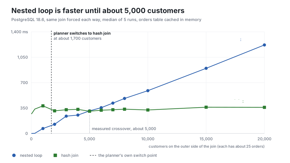
The planner prices the three from estimates, and on the customers-and-orders query the break-even point it worked from was about a third of the one measured. To find the real one, I ran that query at 17 sizes, from 10 customers to all 200,000, and forced each algorithm in turn with enable_hashjoin, enable_mergejoin and enable_nestloop set to off for the session.
| Customers | Orders joined | Nested loop | Hash join | Merge join | Planner’s pick |
|---|---|---|---|---|---|
| 100 | 2,446 | 0.6 ms | 288 ms | 0.6 ms | nested loop |
| 1,000 | 24,899 | 68 ms | 381 ms | 58 ms | nested loop |
| 2,000 | 50,076 | 126 ms | 312 ms | 118 ms | hash join |
| 5,000 | 125,075 | 311 ms | 306 ms | 297 ms | hash join |
| 10,000 | 250,098 | 589 ms | 323 ms | 604 ms | hash join |
| 20,000 | 500,284 | 1,219 ms | 360 ms | 1,451 ms | hash join |
| 50,000 | 1,250,570 | 3,014 ms | 450 ms | 3,083 ms | hash join |
| 200,000 | 5,000,000 | 13,451 ms | 863 ms | 12,511 ms | hash join |
The two cost shapes from the plans explain the whole table. Nested loop pays per customer, about 0.06 ms for each one’s index lookup and page reads, so its line is straight. Hash join pays mostly for one scan of the orders table, so its line is flat. They cross near 5,000 customers, which is 125,000 orders, 2.5 percent of the table. At 200,000 customers the nested loop does 200,000 lookups to fetch every row of a table that a single scan reads in under a second.
Merge join tracks nested loop here, and for the same reason. To get orders in customer_id order it walks the same index, fetching scattered pages one at a time. It came out slightly ahead between 1,000 and 4,000 customers, probably because it walks the index once instead of starting a new search for each customer, and it stops as soon as the customer side runs out, so it never reads the rest of the orders index.
The planner is the surprise. It switched to hash join at 1,721 customers, when its own estimate reached about 1,695, and at 2,000 customers that choice cost 312 ms against 126 ms for the nested loop it rejected. It had the rows right. What it overpriced was the pages: the default random_page_cost = 4 tells it that a page fetched by an index lookup costs four times as much as a page read by a sequential scan, which is roughly right when the page has to come from a disk. In these runs every page was already in memory, so the lookups were much cheaper than the planner assumed.
shared_buffers, so most pages came from the operating system’s cache rather than disk. The jump in nested loop time from 300 customers (1.9 ms) to 1,000 (68 ms) is the point where the pages it touches stop fitting in shared_buffers: the nested loop plan above shows 19,558 pages read from outside it. On a server where those reads go to disk, every nested loop lookup costs more, the crossover moves toward fewer customers, and the planner’s early switch looks much better. Lowering random_page_cost toward 1.1 is the usual advice for SSDs, though the setting applies to every plan on the server at once.That miss cost about two and a half times the time at 2,000 customers. A wrong row estimate errs in the other direction: it can keep a nested loop running long past the line. The PostgreSQL EXPLAIN post showed one source of wrong estimates in this data: the planner treats country and city as unrelated, so it multiplies their selectivities, the fractions of rows each filter keeps. Every city belongs to exactly one country, so the second filter removes nothing the first did not already remove. Here are customers in four countries and those countries’ 40 cities, 16,000 customers in total:
| |
| |
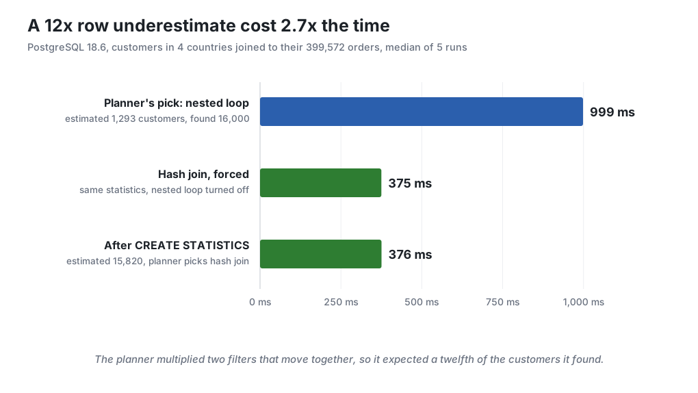
The planner expected 1,293 customers, under its 1,700 switch point, and picked a nested loop. It got 16,000, and the inner side ran 16,000 times. The tell is on the outer side: estimated rows=1293, actual rows=16000.00, and an inner side whose loops matches the actual figure, not the estimate.
| Countries | Estimated customers | Actual customers | Planner’s pick | Nested loop | Hash join |
|---|---|---|---|---|---|
| 2 | 333 | 8,000 | nested loop | 598 ms | 373 ms |
| 3 | 735 | 12,000 | nested loop | 855 ms | 344 ms |
| 4 | 1,293 | 16,000 | nested loop | 999 ms | 375 ms |
| 5 | 2,001 | 20,000 | hash join | 1,206 ms | 358 ms |
| 6 | 2,873 | 24,000 | hash join | 1,442 ms | 380 ms |
The table is the crossover chart again, seen through the estimate. At two to four countries the estimate stays under about 1,700 and the planner keeps the nested loop, up to 2.7 times slower than the hash join. At five countries the estimate crosses 1,700, and the planner switches even though the estimate is still ten times too low. A wrong estimate costs nothing while it stays on the right side of the line.
The fix is to tell the planner the columns are related:
| |
With that, the estimate for four countries went from 1,293 to 15,820 customers, the planner picked the hash join on its own, and the query took 376 ms. MySQL has no equivalent for two columns that share no index (its histograms cover one column each), and with an index on the join column it would not change the join method anyway, for the reason in the MySQL section below.
The quicker reaction to a slow Nested Loop is to turn nested loops off and see what happens. That is a good experiment and a bad fix, because the setting changes every query on the connection, and a nested loop that was slow for 16,000 rows is still the right plan for 16. Christophe Pettus puts it plainly (July 2026): “Diagnose with the switch, then fix the statistics and set it back.”
SET enable_nestloop = off in one session is the quickest way to check whether a hash join would be faster. Leaving it off in postgresql.conf, or in a connection pool’s startup settings, makes every small lookup join in the application pay for a full table scan. With only nested loops off, the 100-customer query took 237 ms as a hash join instead of 0.6 ms. Fix the estimate, then put the setting back.The other obvious fix is memory. Batches above 1 under a Hash node means the hash table spilled to temporary files, as it did in the shipments join, and the natural response is to give it room. I raised work_mem from 1 MB to 1 GB on that join with the hash join forced, and did the same with MySQL’s join_buffer_size:
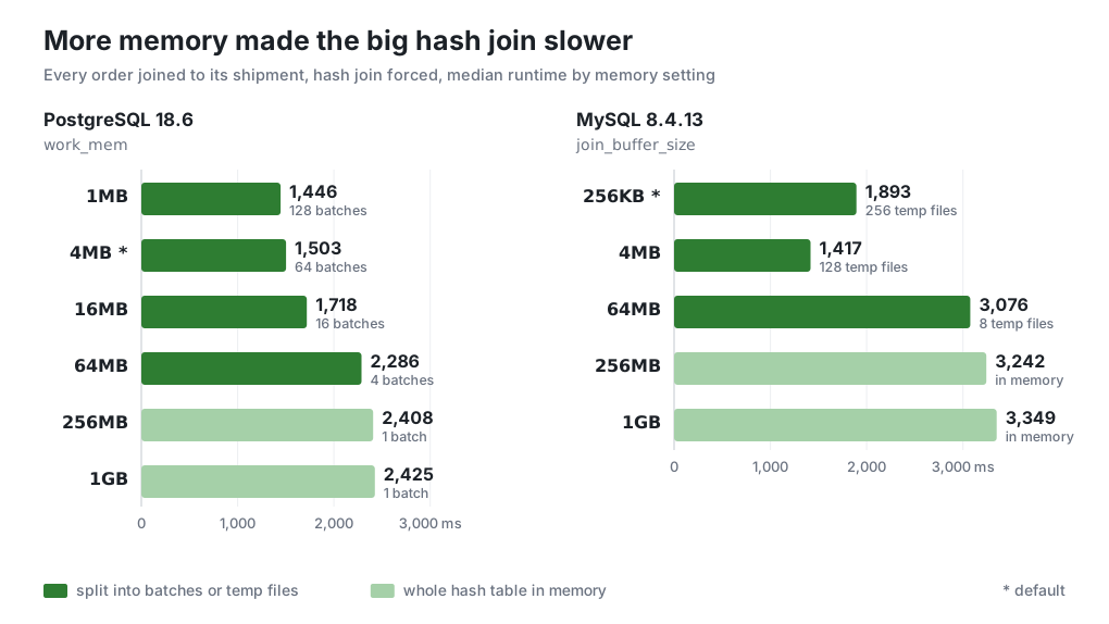
PostgreSQL work_mem | Batches | Hash join | MySQL join_buffer_size | Temp files | Hash join |
|---|---|---|---|---|---|
| 1 MB | 128 | 1,446 ms | 256 KB (default) | 256 | 1,893 ms |
| 4 MB (default) | 64 | 1,503 ms | 4 MB | 128 | 1,417 ms |
| 64 MB | 4 | 2,286 ms | 64 MB | 8 | 3,076 ms |
| 1 GB | 1 | 2,425 ms | 1 GB | 0 | 3,349 ms |
On both engines, the join got slower as it got more memory. In PostgreSQL the single in-memory hash table peaked at 297,571 kB, and the query took 60 percent longer than with 64 small batches. In MySQL the fully in-memory join took more than twice as long as the run that wrote 128 temporary files. I repeated the PostgreSQL runs in a different order, ten runs per setting in all, and the ranking held.
The explanation that fits is the CPU cache. Each probe of a hash table lands at a random spot, and a 290 MB table is far larger than the processor’s cache, so nearly every probe waits on main memory, while a batch of a few megabytes stays in cache for as long as it is being probed. I did not measure cache misses, so treat that as the likely reason rather than a proven one. There is also a caveat that cuts the other way: the temporary files here never reached a disk, since the container had memory to spare and the operating system kept them in its cache. On a server short of memory, where those writes really hit storage, batching costs more.
Small spills still cost something. MySQL’s default 256 KB join buffer is tiny: in the customers-and-orders join it spilled from 8,000 customers on, with 24 temporary files, and took 804 ms against 549 ms with a 4 MB buffer. So a few megabytes helped and a gigabyte hurt. Batches: 64 in a plan says the hash table spilled, which by itself says little about why a query is slow, and Part IV of the queries series covers why raising work_mem server-wide is risky anyway.
MySQL has two of the three, and picks one
MySQL added hash joins in 8.0.18, and in 8.0.20 they replaced the block nested loop, the older method for joining without an index. There is no merge join. The 8.4 manual says when the hash join is used: “for any query for which each join has an equi-join condition, and in which there are no indexes that can be applied to any join conditions.” With an index on orders.customer_id, the optimizer chose the nested loop at every size I tried. To get a hash join I had to hide the index with hints:
| |
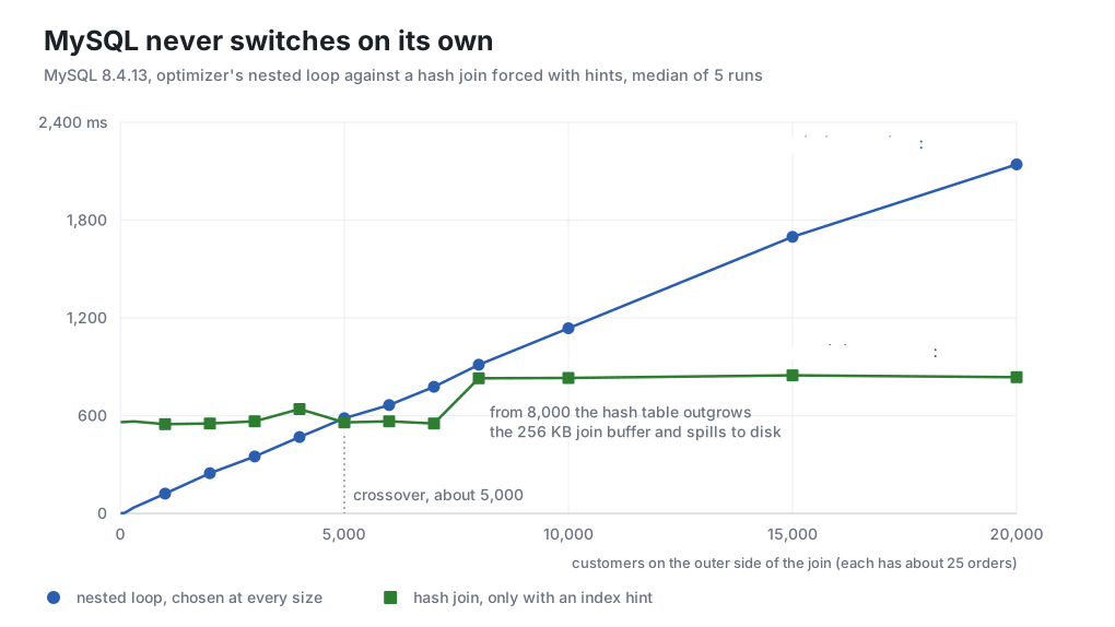
| Customers | Nested loop (optimizer’s pick) | Hash join (forced) |
|---|---|---|
| 1,000 | 121 ms | 548 ms |
| 5,000 | 584 ms | 558 ms |
| 8,000 | 913 ms | 829 ms |
| 20,000 | 2,142 ms | 836 ms |
| 50,000 | 1,084 ms | 869 ms |
| 200,000 | 2,876 ms | 1,237 ms |
The crossover lands near 5,000 customers again, the same place as in PostgreSQL. The difference is that MySQL never makes the switch on its own. Both plans at 20,000 customers:
| |
The cost MySQL printed for the hash join it was forced into is 19.8e+9, against 990,339 for the nested loop. Those are 20,000 times apart, and the runtimes go the other way, 884 ms against 2,149. Whatever the optimizer’s model of a hash join is, it is not one it uses to compete with an index.
What MySQL does change at larger sizes is the join order, which table goes on the outer side. From 50,000 customers on, it starts from the orders table, scanning all 5,000,000 rows once and looking up each order’s customer by primary key. That is still a nested loop, but its cost now grows with the orders scanned instead of the customers selected, which is why 50,000 customers ran faster than 20,000. At 200,000 customers it took 2,876 ms against 1,237 ms for the hash join. (MySQL’s optimizer, to its credit, is very consistent.)
For a reporting query that joins a large share of two big tables, the lever in MySQL 8.4 is an index hint like the one above. Merge join is not available, so the shipments join ran either as a nested loop (2,614 ms) or as a hash join (1,417 to 3,349 ms depending on the buffer).
What to check when a join is slow
Start by naming the join. Each algorithm leaves the same marks in every plan above:
| Algorithm | PostgreSQL plan | MySQL plan |
|---|---|---|
| Nested loop | Nested Loop, with loops= on the inner child equal to the outer side’s rows | Nested loop inner join, with an Index lookup child and its loops= |
| Hash join | Hash Join and Hash Cond, over a Hash child showing Buckets, Batches and Memory Usage | Inner hash join (o.customer_id = c.id), over a Hash child |
| Merge join | Merge Join and Merge Cond, over two inputs in join-column order | does not exist |
Then read its outer side. If estimated rows and actual rows differ by more than a few times, the planner may have chosen for a size it never got, and the inner side’s loops will match the actual number. In PostgreSQL, rerun the query in one session with SET enable_nestloop = off or enable_hashjoin = off. If the other plan is much faster, the algorithm choice was the problem, and the estimate is what to fix: ANALYZE, a higher statistics target on the column, or CREATE STATISTICS for columns that move together. In MySQL the same test is a NO_INDEX hint on the inner table, and with an index on the join column a hint is also the only way to get a hash join.
If the estimate is right and the join is still slow, look at how many rows go into it. A nested loop with 200,000 loops, or a hash join building on millions of rows, is often a query asking for more than the screen shows. Batches above 1 comes last: in these runs a few more megabytes helped and a gigabyte hurt.