How to Read MySQL EXPLAIN ANALYZE Output

TL;DR

EXPLAIN ANALYZE runs your query and shows each step MySQL took to answer it, how long each step took, and how many rows it expected at each step next to how many it got. The habit this post teaches is to find the one slow step first and read only its numbers before changing anything. The output tells you where the time went, not why, and MySQL leaves out some things PostgreSQL shows, so the fix still takes some thinking.

Plain EXPLAIN shows what MySQL plans to do with your query without running it, so every number in it is a guess. EXPLAIN ANALYZE runs the query for real and prints the same plan with what happened at each step: rows out, time taken, and how many times the step ran. A plan can look sensible and still read the whole table, and only the second command shows that. You can paste the output into an AI and get a reading back, and it will often point at the right line. What it does not know is your system: which table is the busy one, what the query is for, whether a number that looks large is normal here. That judgment is yours, and this post is about having enough of it to check the reading rather than take it.

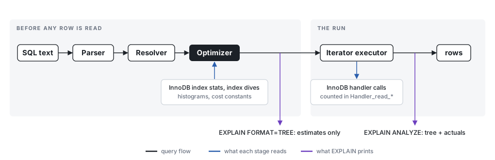
The part of MySQL that decides how to run a query is the optimizer, and it decides before reading any data. It lists the ways it could answer (read the whole table or use an index, which table to start a join with), estimates the cost of each, and picks the cheapest. Its estimates come from statistics InnoDB keeps about each table and its indexes, and from quick samples of an index taken while planning. When a column has no index, the optimizer knows very little about it and falls back on rough rules. That is why plain EXPLAIN answers instantly, and why it can be badly wrong.

The executor then runs the chosen plan and counts what happens. EXPLAIN ANALYZE prints those counts next to the optimizer’s guesses, and reading it mostly means comparing the two.

SQL passes through the parser, resolver and optimizer before any row is read; the iterator executor then runs the plan. EXPLAIN prints the plan with estimates, EXPLAIN ANALYZE adds what actually happened

Every plan below comes from MySQL 8.4.13 in Docker with default settings, on a customers table of 200,000 rows (50 countries, 10 cities each) and an orders table of 5,000,000. Each order belongs to a random customer, so one customer’s orders are scattered across the table, the way real orders arrive. The PostgreSQL version of this post uses the same rows.

What the output is telling you

Start with the simplest slow query there is: one customer’s orders, before any index exists on customer_id.

1
SELECT id, created_at, total FROM orders WHERE customer_id = 4242;

EXPLAIN FORMAT=TREE prints the plan as a tree:

1
2
-> Filter: (orders.customer_id = 4242)  (cost=529407 rows=496280)
    -> Table scan on orders  (cost=529407 rows=4.96e+6)

Each line starting with -> is one step. MySQL calls a step an iterator, because each one hands rows, one at a time, to the step above it. The deeper a line is indented, the earlier it runs, so read from the innermost line out. Table scan on orders means read every row of the table from start to finish. Its rows go up to Filter, which is the WHERE condition, checked against each row. rows= is the estimate: about 4.96 million rows from the scan (4.96e+6 is engineering notation for 4,960,000), and 496,280 expected to match. cost is the optimizer’s price in its own units, not milliseconds. Now with EXPLAIN ANALYZE:

1
2
-> Filter: (orders.customer_id = 4242)  (cost=529407 rows=496280) (actual time=16.7..652 rows=27 loops=1)
    -> Table scan on orders  (cost=529407 rows=4.96e+6) (actual time=0.224..578 rows=5e+6 loops=1)

The first parenthesis is still the guess. The second is what happened. actual time=0.224..578 on the table scan is milliseconds until it produced its first row and its last row. rows=5e+6 is the rows it produced: all five million. loops=1 is how many times the step ran, which matters later. On the Filter, rows=27 is how many matched, against a guess of 496,280.

Two things are wrong here, and they are different problems. The guess was off by a factor of 18,000, which is a lot even for a guess. With no index on customer_id the optimizer had little to go on, and its guess works out to exactly a tenth of the table. And even a perfect guess would not have helped, because without an index there was no faster way to find 27 rows than reading all five million. That is what the table scan’s rows=5e+6 says, and on a slow query it is the first number worth finding.

An index is that faster way. It is a separate sorted structure, like the index at the back of a book, that maps each customer_id to where that customer’s rows are stored. After CREATE INDEX orders_customer_id_idx ON orders (customer_id):

1
-> Index lookup on orders using orders_customer_id_idx (customer_id=4242)  (cost=28.7 rows=27) (actual time=0.044..0.0452 rows=27 loops=1)

One step, a lookup instead of a scan. The guess is now exactly right (rows=27), because the index gives the optimizer real numbers to work from, and the query takes 0.045 ms instead of 652.

EXPLAIN ANALYZE really runs the query

For a SELECT it takes as long as the query takes; the MySQL manual notes you can stop it with KILL QUERY or Ctrl-C. It also accepts some UPDATE and DELETE statements, so treat it as running them and wrap it in START TRANSACTION; and ROLLBACK;. Run long queries on a copy or a replica, not the server your users are on.

When the database guessed wrong

When the optimizer guesses wrong it can pick the wrong plan, so the estimate is worth checking on every slow step. This query joins the two tables (a join matches rows in one table to rows in another, here customers to their orders) and totals the orders of every customer in one city:

1
2
3
4
SELECT count(*), sum(o.total)
FROM customers c
JOIN orders o ON o.customer_id = c.id
WHERE c.country = 'C07' AND c.city = 'C07-3';

1
2
3
4
5
-> Aggregate: count(0), sum(o.total)  (cost=75057 rows=1) (actual time=84.4..84.4 rows=1 loops=1)
    -> Nested loop inner join  (cost=70156 rows=49011) (actual time=0.222..84 rows=9940 loops=1)
        -> Filter: ((c.city = 'C07-3') and (c.country = 'C07'))  (cost=20384 rows=2001) (actual time=0.103..29.8 rows=400 loops=1)
            -> Table scan on c  (cost=20384 rows=200070) (actual time=0.0927..22.6 rows=200000 loops=1)
        -> Index lookup on o using orders_customer_id_idx (customer_id=c.id)  (cost=22.4 rows=24.5) (actual time=0.127..0.135 rows=24.9 loops=400)

Read it inside out. The deepest line, Table scan on c, reads all 200,000 customers. Filter keeps the ones in that city: it expected 2,001 and found 400. That is the thing to look for, estimated rows against actual rows on the same line. Neither column has an index, and the guess again works out to a tenth per condition: a tenth of a tenth of 200,070 is 2,001.

Nested loop inner join is one way to do a join. It has two children at the same depth: the first (the filtered customers) runs once, and for each row it produces, the second (find that customer’s orders through the index) runs once. That is what loops=400 on the Index lookup means. When loops is above 1, rows and actual time are averages per run, so multiply them back: 24.9 rows times 400 is the 9,940 rows the join produced, and 0.135 ms times 400 is 54 ms, most of the 84. The join’s own estimate was 49,011 rows against 9,940, the first mistake carried up the tree.

Here the wrong guess did no harm, because with 2,001 customers or 400, looking up each one’s orders in the index is a good plan. A gap matters when the right number would have made the optimizer choose differently, and the bigger the gap, the more likely that is. The next section has one where a wrong guess fed into a choice of index.

When the plan is fine but still slow

The first plan already showed the second lesson: a scan that read the whole table, given away by rows=5e+6 on the Table scan line. Here it is in a bigger tree to practice on, the 100 largest orders since November 1 with each customer’s location:

1
2
3
4
5
6
SELECT o.id, o.total, c.country, c.city
FROM orders o
JOIN customers c ON c.id = o.customer_id
WHERE o.created_at >= '2024-11-01'
ORDER BY o.total DESC
LIMIT 100;

1
2
3
4
5
6
-> Limit: 100 row(s)  (cost=2.29e+6 rows=100) (actual time=789..789 rows=100 loops=1)
    -> Nested loop inner join  (cost=2.29e+6 rows=4.96e+6) (actual time=789..789 rows=100 loops=1)
        -> Sort: o.total DESC  (cost=529519 rows=4.96e+6) (actual time=789..789 rows=100 loops=1)
            -> Filter: (o.created_at >= TIMESTAMP'2024-11-01 00:00:00')  (cost=529519 rows=4.96e+6) (actual time=585..675 rows=608001 loops=1)
                -> Table scan on o  (cost=529519 rows=4.96e+6) (actual time=0.114..572 rows=5e+6 loops=1)
        -> Single-row index lookup on c using PRIMARY (id=o.customer_id)  (cost=0.997 rows=1) (actual time=0.0054..0.00541 rows=1 loops=100)

Each step’s time includes the time of the steps under it, so to see what one step cost by itself, subtract its children’s finishing times from its own. Sort finished at 789 ms and its child at 675, so sorting cost 114 ms. Filter finished at 675 and the scan under it at 572, so checking the dates cost 103. Table scan on o cost 572 ms by itself, more than everything else put together. It read five million rows to keep 608,001. The customer lookups ran 100 times at 0.0054 ms each, half a millisecond in all.

Two more things are visible once you know where to look. The Sort produced its first row at the same moment as its last (789..789), because a sort cannot hand anything up until it has seen all its input. And the Filter produced its first row at 585 ms, because the newest orders sit at the end of the table and the scan reaches them last.

There was an index on created_at while this ran, and MySQL did not use it. It estimated about 1.27 million matching rows (the real number was 608,001), and priced 1.27 million trips from the index back to the table as dearer than one pass over the whole table. The guess was off by half; the plan alone cannot say whether the right number would have changed the choice. An index that holds every column the query needs never makes those trips. After CREATE INDEX orders_created_total_cust_idx ON orders (created_at, total, customer_id):

1
2
3
4
5
6
-> Limit: 100 row(s)  (cost=1.49e+6 rows=100) (actual time=183..183 rows=100 loops=1)
    -> Nested loop inner join  (cost=1.49e+6 rows=1.28e+6) (actual time=183..183 rows=100 loops=1)
        -> Sort: o.total DESC  (cost=258614 rows=1.28e+6) (actual time=183..183 rows=100 loops=1)
            -> Filter: (o.created_at >= TIMESTAMP'2024-11-01 00:00:00')  (cost=258614 rows=1.28e+6) (actual time=0.0673..73.8 rows=608001 loops=1)
                -> Covering index range scan on o using orders_created_total_cust_idx over ('2024-11-01 00:00:00' <= created_at)  (cost=258614 rows=1.28e+6) (actual time=0.0669..54.9 rows=608001 loops=1)
        -> Single-row index lookup on c using PRIMARY (id=o.customer_id)  (cost=0.862 rows=1) (actual time=0.00143..0.00145 rows=1 loops=100)

Covering index range scan means MySQL read only the part of the index from November 1 onward, and found everything it needed there. 183 ms instead of 789. The sort is now the slowest step at 109 ms, and that part is the price of the question: finding the 100 largest of 608,001 orders means looking at all 608,001. The new index costs something too, 152 MB on disk and extra work on every insert, so it is worth it for a query that runs often and maybe not for a nightly report.

Next thing to learn: counting what MySQL read

PostgreSQL’s plan prints how many pages each step read. MySQL’s does not, and it does not say when a sort spilled to disk either. Session status counters fill part of the gap: run FLUSH STATUS, then the query, then SHOW SESSION STATUS LIKE 'Handler_read%'. For the one-customer query without an index, Handler_read_rnd_next was 5,000,001, one per row scanned. With the index, it was 0, and Handler_read_next was 27.

What the warning signs mean

Table scan under a Filter that keeps a small share of its rows means MySQL read the whole table to find a few. The usual fix is an index on the WHERE column. If one exists and goes unused, check whether the condition wraps the column in a function, which hides it from the index; Non-SARGable Predicates explains that one.

Index range scan or Index lookup where you might have had Covering index range scan means MySQL found the rows in the index, then went back to the table for each one to fetch the other columns. Counting 25,182 orders for a range of customers took 2.3 ms as a covering scan. Summing their total, a column not in the index, took 95 ms. Adding the missing column to the index is the usual fix, with the size cost above.

Nested loop inner join with a large loops on its second child means one lookup repeated many times. Fine when the repeated step is an index lookup, as in both joins above. When it is a Table scan, the join column has no index and the whole table is read once per loop.

A Sort with a large input means every row has to be read before the first one comes out. If the sort is the slow step, ask whether the query needs all those rows. The tree will not tell you whether it spilled to disk.

The first five things to look at

The top line’s last time: the number you want smaller.
The slowest step. From the top, subtract each step’s children from its own finishing time until you find the step that is slow by itself.
On that step, actual rows against the estimate. A big difference means the optimizer guessed wrong.
Under that step, a Table scan whose rows is close to the table’s size, when only a few rows survive. That means a missing index.
Rows handled against rows needed. Thousands sorted for a page of 100 means the query asks for more than the question.

When you are ready for a real one, A Query on a 3-Billion-Row Table Took 100 Minutes reads a production MySQL plan end to end the same way.

The ways MySQL reads a table

Every leaf of the tree is one of a short list of access methods, and the name says how much of the table or index MySQL expects to touch. The older EXPLAIN output, the one without FORMAT=TREE that most tutorials still show, names the same methods in its type column, so both are listed. Rows are ordered from cheapest to most expensive. The names below were taken from MySQL 8.4.13 on a small separate schema, since the post’s own fixture does not produce all of them.

What the tree says	`type` in classic EXPLAIN	What MySQL does	What it usually means
`Rows fetched before execution`	`const`	Looked up one row by primary key or unique index while planning; the row is a constant by the time the query runs	As good as it gets
`Single-row index lookup on t using PRIMARY (id=...)`	`eq_ref`	For each row from the previous step, one lookup that returns at most one row	The normal shape of a join on a primary key
`Index lookup on t using k (col=...)`	`ref`	Finds every row with one value through a non-unique index, then fetches each row from the table	Fine when `rows` is small; expensive when one value matches thousands
`Covering index lookup on t using k (col=...)`	`ref` + `Using index`	Same lookup, but every column the query needs is in the index, so the table is never read	Cheaper than a plain lookup; adding a column to the SELECT can turn it back into one
`Index lookup ... (col=... or NULL)`	`ref_or_null`	A lookup that also fetches the rows where the column is NULL	A `col = x OR col IS NULL` condition
`Index range scan on t using k over (a < col < b)`	`range`	Walks the part of the index between two bounds, fetching rows from the table	Normal for date ranges; watch `rows` against what the query returns
`Covering index range scan on t using k over (...)`	`range` + `Using index`	The same walk without touching the table	The cheapest range
`Sort-deduplicate by row ID` over two range scans	`index_merge`	Runs two index scans and combines their row IDs	An `OR` across two indexed columns; often slower than it looks
`Index scan on t using k`	`index`	Reads the whole index in order and fetches every row from the table	Usually an `ORDER BY` on an indexed column with no filter; expensive when the table is large
`Covering index scan on t using k`	`index` + `Using index`	Reads the whole index without the table	Cheaper than a table scan because the index is smaller, still every row
`Table scan on t`	`ALL`	Reads every row in the table	The one to look for when a query is slow and only a few rows survive the `Filter` above it
`Zero rows (Impossible WHERE)`	`Impossible WHERE`	The optimizer proved no row can match and reads nothing	A condition that contradicts itself

A few more names appear above the leaves and describe what happens to rows once they are read. Filter: keeps the rows that pass a condition the index could not check. Nested loop inner join runs its second child once per row from the first, which is where loops comes from. Inner hash join reads the smaller side once into memory and probes it, and the classic output shows it as Using join buffer (hash join). Sort: orders rows in memory or in a temporary file, which the plan does not distinguish. Limit:, Group aggregate: and Aggregate: do what their names say, and Materialize writes an intermediate result to a temporary table that a Table scan above it then reads.

The test data was generated once with PostgreSQL (the script is at the end of the PostgreSQL post), exported to CSV, and loaded into these tables on MySQL 8.4:

 1
 2
 3
 4
 5
 6
 7
 8
 9
10
CREATE TABLE customers (id int PRIMARY KEY, country varchar(8) NOT NULL,
                        city varchar(16) NOT NULL, created_at datetime NOT NULL);
CREATE TABLE orders (id bigint PRIMARY KEY, customer_id int NOT NULL,
                     status varchar(16) NOT NULL, created_at datetime NOT NULL,
                     total decimal(10,2) NOT NULL, note text);
LOAD DATA INFILE '/var/lib/mysql-files/customers.csv' INTO TABLE customers
  FIELDS TERMINATED BY ',' (id, country, city, created_at);
LOAD DATA INFILE '/var/lib/mysql-files/orders.csv' INTO TABLE orders
  FIELDS TERMINATED BY ',' (id, customer_id, status, created_at, total, note);
ANALYZE TABLE customers, orders;